Documentation of Cloud Tracking Algorithm

Introduction

The cloud tracking algorithm presented here builds upon the Iterative Rain Cell Tracking (IRT) algorithm developed by Moseley and Haeter in 2020. We have expanded this approach from tracking 2-dimensional rain cells to capturing 3-dimensional cloud objects in the cloud resolving model.

This algorithm is designed to track the liquid water path instead of rain cells, projecting the identified entities onto the 3-dimensional cloud objects. For the sake of simplicity and ease of operation, when addressing the merging and splitting of cloud objects during their time evolution, we treat them as the same identity. (Refer to the detailed process outlined below.)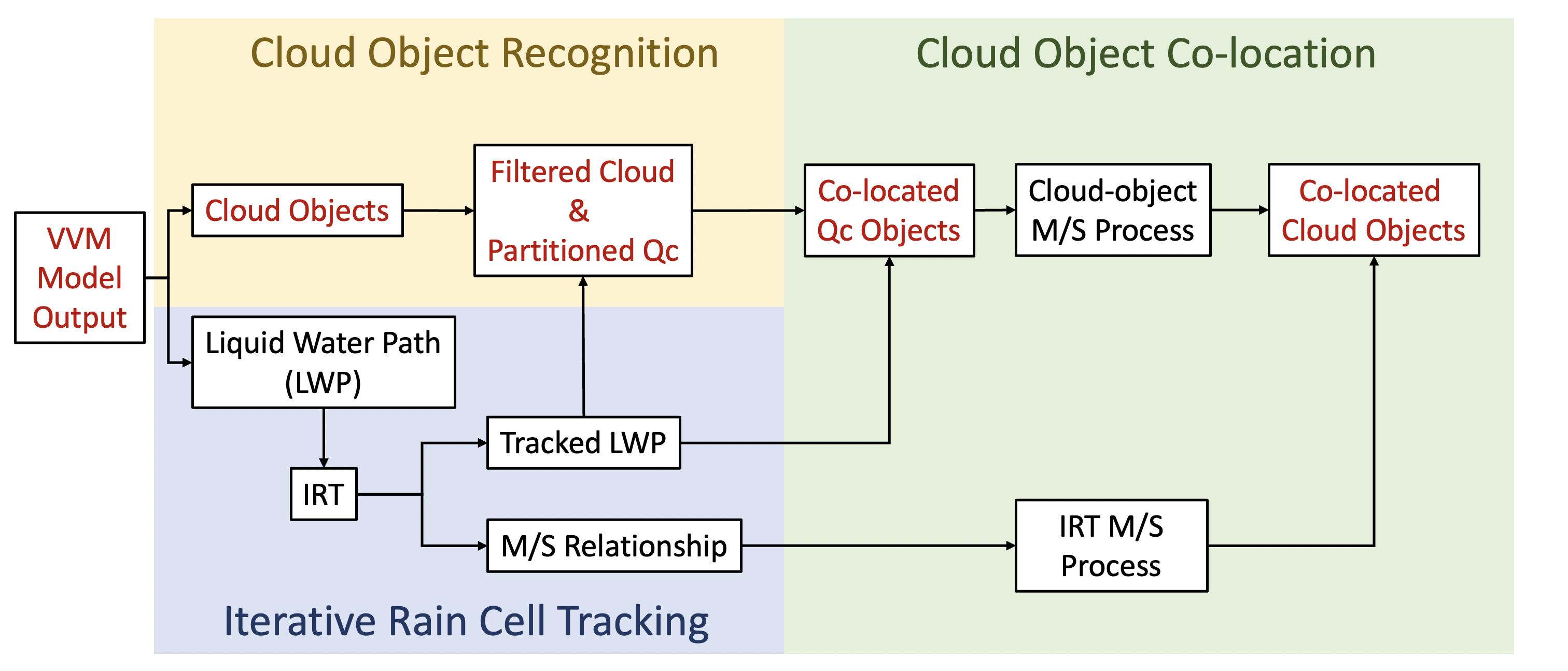

Table of Contents:

• Source Code: https://github.com/neko2048/iterativeRainCellTracking
• Iterative rain cell tracking
  • Parameter Setup
  • Transfer 2D Track Variable
  • Main Program
  • Merge All Parent & Children Track ID to Same Track ID
  • Project Track ID to LWP Regions
• Cloud Water Object Recognition & Filtering
  • Cloud Object Recognition
  • Cloud Object Filtering
  • Qc Object Recognition
  • Qc in Same Cloud Identification
• Qc Co-location
  • Collocate Qc Objects
  • Merge Multiple LWP if they overlaps with one Qc
• Map Qc to Cloud
  • Map Qc to Cloud

Iterative rain cell tracking

1. Parameter Setup:

   RRtrack/
    |- irt_parameters_fskao.f90
   

   Modify irt_parameters_fskao.f90 to set up the parameters. For current step, I tracked liquid water path (LWP) with a threshold of 2.5 g/kg.
   In my experience, max_no_of_cells, max_no_of_tracks, and max_length_of_track cannot be too large, and threshold cannot be too small. Otherwise, the system could print out error when executing do_iterate.sh.

2. Transfer 2D Track Variable

   RRtrack/
    |- do_transfer.sh
    |- transfer.f90
   

   Program for transferring .nc file to .srv file.

3. Main Program

   RRtrack/
    |- do_iteration.sh
   

   Main program for generating tracking data.

4. Merge All Parent & Children Track ID to Same Track ID.

   cloudTracking/mergeSplitIRT/
    |- saveTrackLinks_v2.py
   

   Merge all parent & children track ID to same track ID.

5. Project Track ID to LWP Regions

   cloudTracking/mergeSplitIRT/
    |- lwpCollocate.py
   

   Project track ID to LWP regions.

Cloud Water Object Recognition & Filtering

1. Cloud Object Recognition

   cloudTracking/cloudObject/
    |- cloudObject2nc_2layer.py
   

   Recognize cloud objects with a given condition by six-connected segmentation method. Currently, we take two selecting condition as the fact that only condition (2) might leads to overestimated of cloud base height and only condition (1) leads to no anvil ($q_c$ existence reaches to about 10 km only).
   (1) \(q_c > 0\)
   (2) \(q_c + q_i \leq 10^{-4} kg\ /\ kg\)

2. Cloud Object Filtering

   cloudTracking/cloudFilter/
    |- cloudObjectFilter_2Layer.F
   

   Filter out the cloud objects that are too high (e.g. cloudbase > 1000) and too thick (e.g. cloudDepth < 500)

3. Qc Object Recognition

   cloudTracking/cloudObject/
    |- qcExtractor.py
   

   Extract qc objects from filtered cloud objects.

4. Qc in Same Cloud Identification

   cloudTracking/qcCollocate/
    |- qcCollocate.py
   

   If multiple qc objects belong to one cloud, then assign them same label.

Qc Co-location

1. Collocate Qc Objects

   cloudTracking/qcCollocate
    |- collocateQc_v3.py
   

   Map LWP regions with track ID to qc objects and record if one 1 qc overlaps with multiple LWP regions.

2. Merge Multiple LWP if they overlaps with one Qc

   cloudTracking/mergeSplitIRT/
    |- mergeHistoryTrack.py
   

   Merge Multiple LWP if they overlaps with one Qc.

Map Qc to Cloud

1. Map Qc to Cloud

   cloudTracking/assignCloudIndex/assignCloudIdx.py
   

   Map Qc to Cloud